6.1. R: Introduction to R
The standard installation of R utilizes a default user interface. In this course, we will instead use RStudio which provides a richer interface. Once you have installed the R base package, download RStudio from the following website: http://www.rstudio.com/.
R is an open source package. This has both advantages and disadvantages. Because it is open source, there is no “software support” you can directly access; however, there are literally thousands of documents on the web that can help you use R efficiently (some are much better than others). The following links give some of the most popular webpages for R support.
- http://cran.r-project.org/other-docs.html
- http://cran.r-project.org/manuals.html
- http://cran.r-project.org/doc/manuals/R-intro.html
R’s base package contains many basic functions used in statistics. In addition to the base package, many individuals have created other packages that can be downloaded that will aid in various analyses.
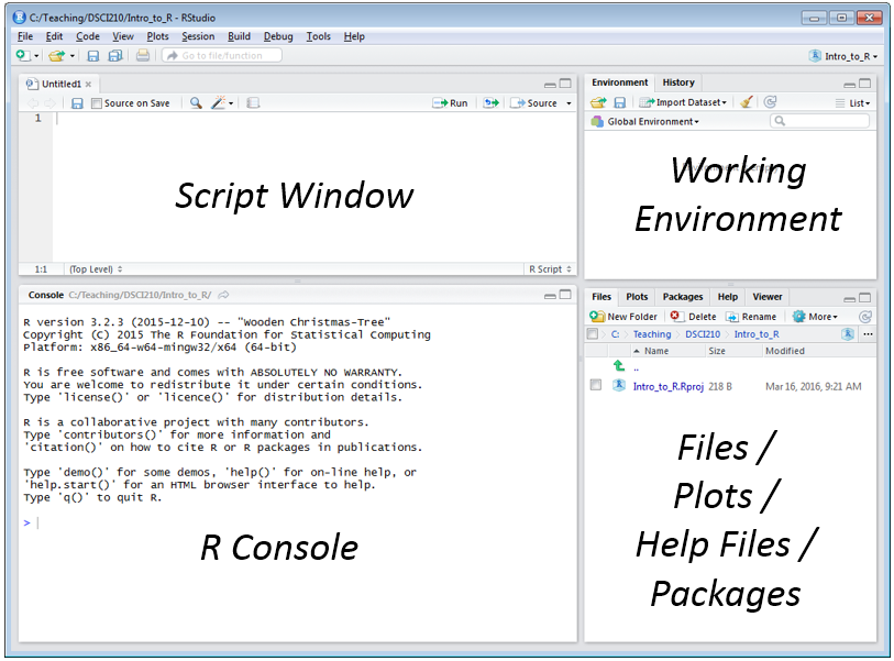
The following provides a snapshot of the R Studio interface that is commonly used when using R.
Organizational Structure
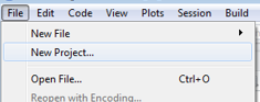
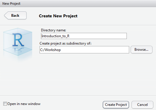
The organization structure in R is best managed through what is called Projects. To create a new Project, select File > New Project …
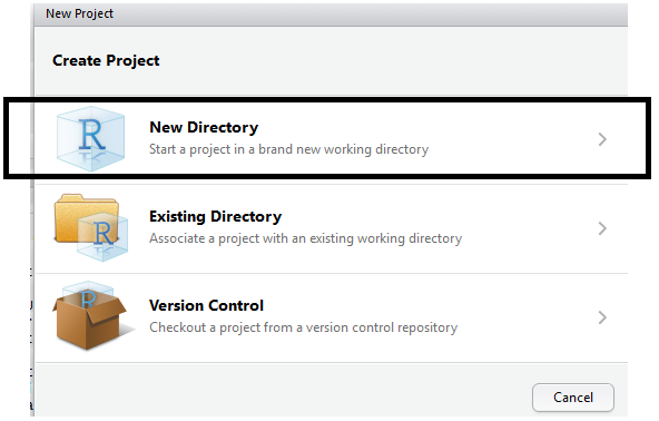
First, specify New Directory
|
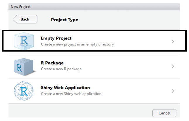
Next, to begin we will create an Empty Project
|
Specify the name and location for the new directory that will contain this new project.
Next, specify the name and location fo this new directory
|
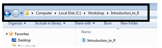
Verify that the new direcory and project has been created
|
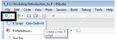
The frame in the upper-left is your script window and the frame on the lower-left is the R console window. You can enter command directly into the R console; however, I’d encourage you to get accustomed to using the script window. The following can be used to obtain an R script window.
*Reading Data Files into R Studio*
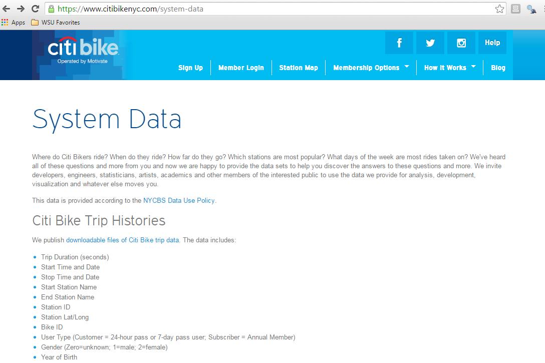
Citibike is a bike rental company that operates in New York City. Citibike bike rental data is publically available.
- Citibike: https://www.citibikenyc.com/
- System Data: https://www.citibikenyc.com/system-data
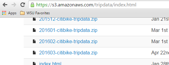
- Amazon data download: https://s3.amazonaws.com/tripdata/index.html
 |
 |
Scroll down and save a copy of the most recent dataset onto your local machine.
Unzip the file that you’ve downloaded from this website. A comma delimited text file is produced.
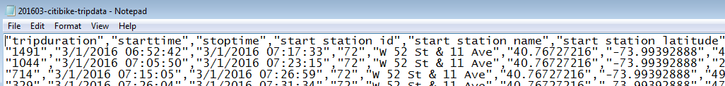
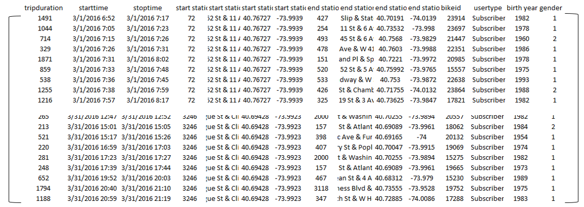
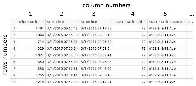
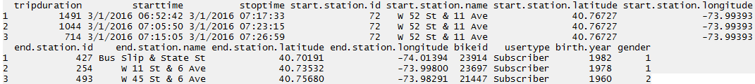
The Citibike dataset is highly structured. The first row contains the variable or field names. Each row represents a single instance of a bike rental.
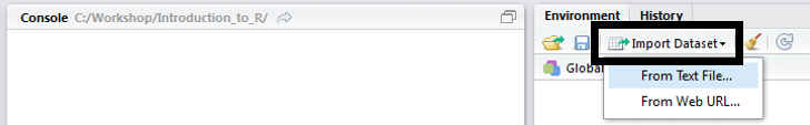
To open a text file in RStudio, select Import Dataset in the window shown in the upper-right. Choose to import data from a Text File.
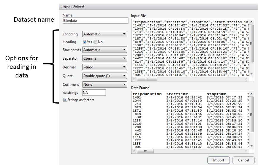
Select the text file to be read in. The Citibike bike rental dataset is being read in here. Give a name to the dataset in the Name box. Options may need to be specified, the default setting suffice for this dataset.
*Understanding Data Objects*
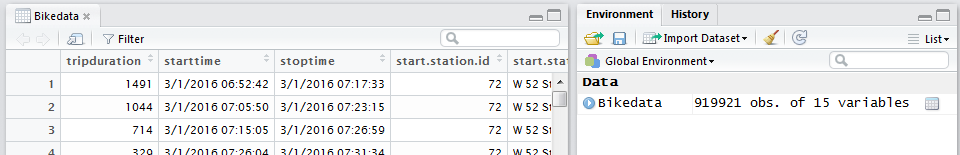
Click Import, and the data set will be added to your workspace. If you click on the data set name in your workspace, the data set will appear in the upper-left window.
R is an object oriented language and there are a few basic objects used to store data. In an effort to keep things simple, consider the following explanations.
- vector: the contents of a single column
- data.frame: a collection of vectors – restricted to each having same length
- list: a collection of vectors
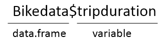
R stores the imported data in an object known as a data frame. The type of object can be identified using the class() function.
> class(Bikedata)
[1] “data.frame”
The str() function can be used to provide additional details regarding an object.
> str(Bikedata)
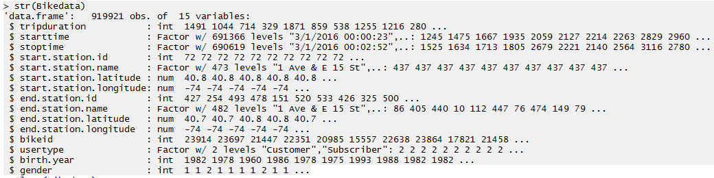
Questions:
- How many observations, i.e. rows, does Bikedata contain?
- How many variables, i.e. columns, doe the Bikedata contain?
A data.frame may contains a mix of data types. From the above output, we can see that tripduration is an integer, start.station.latitude is a number, and strings are identified as factors. A factor variable has levels inherently defined – which is beneficial when summarizing data.
The summary() function is a generic function that produces summaries that are relevant to the object being passed into the function.
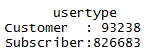
> summary(Bikedata)
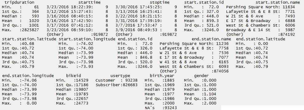
Consider the following summaries provided above.
Summaries for a numeric variable
Measurement Units: Seconds |
Summaries for a factor
|
Questions:
- Provide a brief description of the summary statistics for tripduration. What information about bike rentals in NYC do these summaries provide?
- Provide a brief description of the summary statistics for usertype. What information about bike rentals in NYC do these summaries provide?
*Creating New Objects*
R allows one to easily work with individual variables within a data.frame.
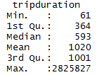
For example, the str() and summary() function can be applied only the tripduration variable
> str(Bikedata$tripduration)
int [1:919921] 1491 1044 714 329 1871 859 538 1255 1216 280 ...
>
> summary(Bikedata$tripduration)
Min. 1st Qu. Median Mean 3rd Qu. Max.
61 364 593 1020 1001 2826000
R allows us to easily create a new variable. The “<-“ is the assignment operator and is used to assign output to an object. R attempts to identify the most appropriate object type when assignments are made. The following will convert the trip duration to minutes. The outcome will be placed into an object called trip.minutes.
> trip.minutes <- Bikedata$tripduration / 60
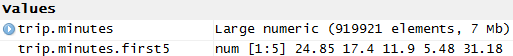
Notice that a new (vector) object is created.

Once again, the structure of this object can be identified using str(). A summary of this newly created vector is provided here as well.
> str(trip.minutes)
num [1:919921] 24.85 17.4 11.9 5.48 31.18 ...
Min. 1st Qu. Median Mean 3rd Qu. Max.
1.02 6.07 9.88 17.00 16.68 47100.00
A new object can be assigned to directly to an existing data.frame as follows.
> Bikedata$trip.minutes <- Bikedata$tripduration / 60
The number of variables in the Bikedata data.frame before creating this new variable.

The number of variables in the Bikedata data.frame after creating this new variable.

*Referring to Elements of Objects - Vectors*
As seen above, R allows us to create a new variable from an existing column within a data.frame. R also allows us to obtain certain segments (or subsets) of data objects as well.
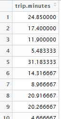
trip.minutes is stored as a vector within R
|
Prettified version of
trip.minutes
|
The bracket syntax, i.e. [ ], is used to refer to particular segments of data objects. For example, the get the 1st element of the trip.minutes vector, trip.minutes[1] is used. The second element is obtained simple by changing the 1 to a 2.
> trip.minutes[1]
[1] 24.85
> trip.minutes[2]
[1] 17.4
The first five elements can be obtained using 1:5 as is shown here.
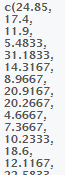
> trip.minutes[1:5]
[1] 24.850000 17.400000 11.900000 5.483333 31.183333
If the first five elements are to be saved into a new object, simply make the necessary assignment.
> trip.minutes.first5 <- trip.minutes[1:5]
A new vector of length five is created in your environment.
The length() function can be used to identify the number of elements in a vector.
> length(trip.minutes.first5)
[1] 5
Note: The analogous function for a data.frame is nrow(), or the function dim() can be used as well.
*Referring to Elements of Objects – data.frames*
For a data.frame, names can be specified for the rows and columns. Generally speaking, column names are more important as these are used to identify fields or variables within the dataset. The colnames() and rownames() functions can be used to identify column names and row names, respectively.
> colnames(Bikedata)

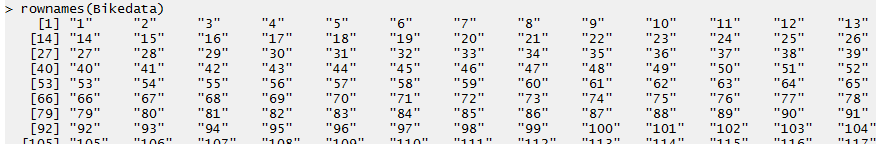
> rownames(Bikedata)
Akin to vectors, R allows one to refer to rows and columns by number as well.
Once again, the square bracket syntax is used to refer to particular segments of data objects. The data.frame is a two-dimensional object; thus, a row and column identifier can be specified.
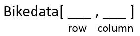
Getting the 1st row, 1st column of Bikedata
> Bikedata[1,1]
[1] 1491
Getting the 1st three rows and only the 1st column of Bikedata
> Bikedata[1:3,1]
[1] 1491 1044 714
Getting the 1st three rows and 1st three columns of Bikedata
> Bikedata[1:3,1:3]
tripduration starttime stoptime
1 1491 3/1/2016 06:52:42 3/1/2016 07:17:33
2 1044 3/1/2016 07:05:50 3/1/2016 07:23:15
3 714 3/1/2016 07:15:05 3/1/2016 07:26:59
Getting the 1st three rows and all columns of Bikedata. If the column argument is not specified, then all columns are provided.
Bikedata[1:3 , ]
> Bikedata[1:3,]
Getting the 1st three rows and only columns 1, 4, and 5. The c( ) syntax is used to create a new vector object. The vector simple specifies which columns to retain in this subset of Bikedata.
Bikedata[1:3 , c(1,4,5) ]
> Bikedata[1:3,c(1,4,5)]
tripduration start.station.id start.station.name
1 1491 72 W 52 St & 11 Ave
2 1044 72 W 52 St & 11 Ave
3 714 72 W 52 St & 11 Ave
*Getting Help with R*
Within R, you can find help on any command (or find commands) using the following.
If you know the name of the R function, e.g. summary, use help(summary) or ?summary.
> help(“summary”)
> ?summary
If you don’t know the function and want to do a keyword search for it, use help.search().** **
> help.search(“summary”)
The help.start() function will launch the full help system that includes all manuals, references, etc.
> help.start()