6.9. Classification Trees in R¶

A classification tree is an example of a simple machine learning algorithm – an algorithm that uses data to learn how to best make predictions. Classification trees can be applied to a large class of problems, e.g. to determine whether or not a credit card transaction is fraudulent or to determine whether or not someone has cancer.

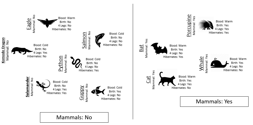
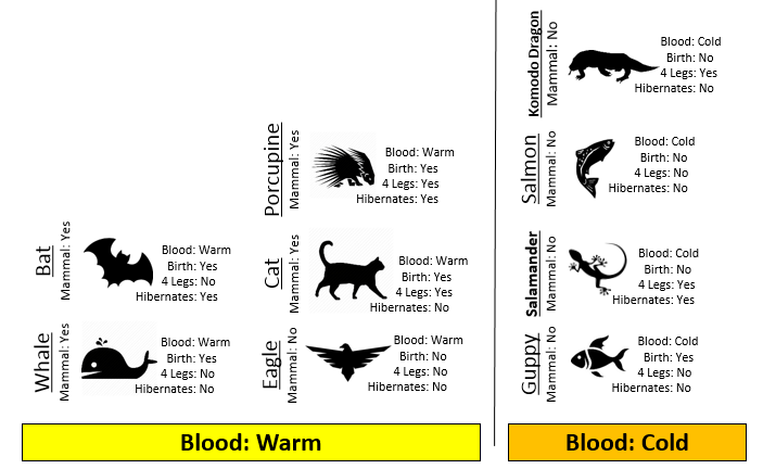
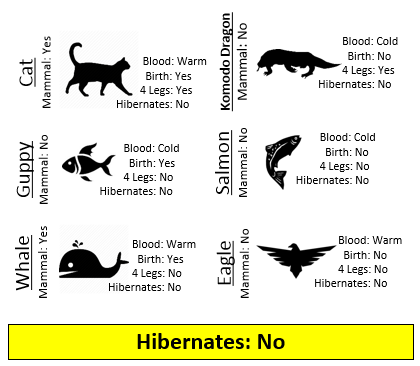
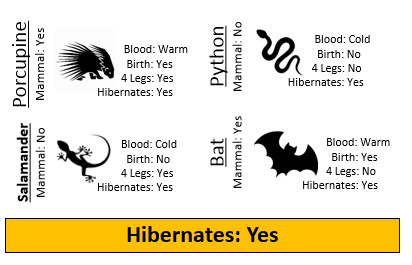
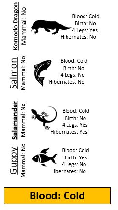
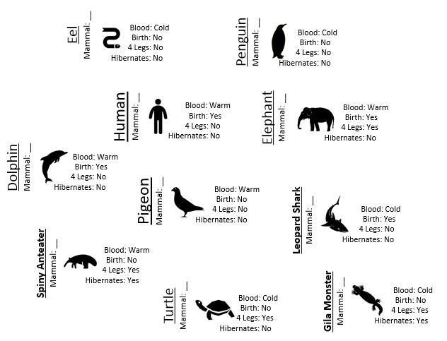
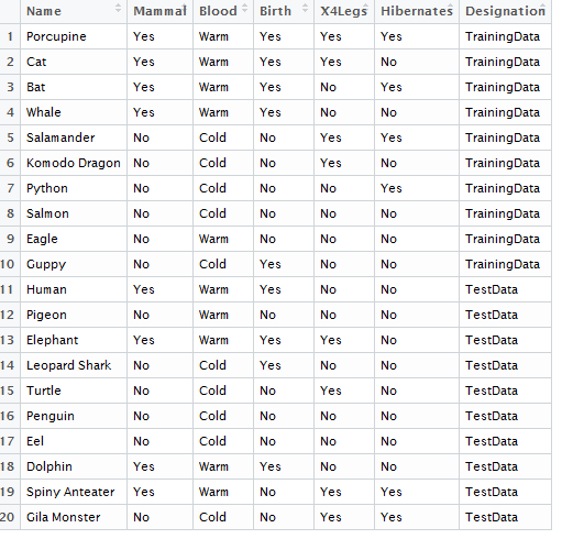
Example 8.1: Consider the following animals. The machine learning goal here is to separate (or classify) these animals into two groups – mammals and non-mammals.

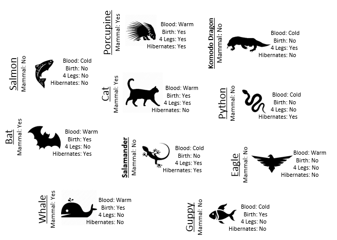
The most obvious way to separate/classify these animals is divide the groups based on whether or not the animal is a mammal. However, this approach has absolutely no predictive ability because you are using the outcome to predict the outcome. This would be akin to placing a beat on the Super Bowl in Las Vegas after the Super Bowl has been played.

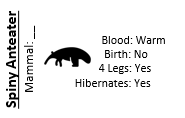
The approach taken above does not allow us to make prediction for a new mammal, say a Spiny Anteater.

Tasks

1. Visit the course website, click on the Training web link. Use the four predictor variables: 1) Blood (Warm/Cold), 2) Gives Birth (Yes/No), 3) 4 Legs (Yes / No), and 4) Hibernates (Yes / No) to build a set of rules for classifying each animal as a mammal or non-mammal. Briefly describe your process below.
2. Next, click on the Test web link. Apply the rule you developed above to classify each of the animals provided here. How well did your rule work? Discuss.
3. Compare and contrast your rule against a classmate. Which rule is better – yours or theirs? How did you define “better”? Discuss.

Development of a Classification Rule

Machine learning requires that the methodology being used makes predictions in a logical, systematic, and precise manner.

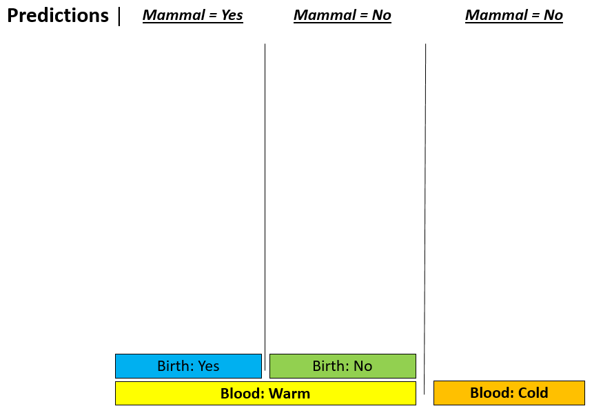
Consider the following two rules for classifying animals into Mammals and Non-mammals.

	Rule #1: Hibernates > Blood > Give Birth	Rule #2: Blood > Give Birth
Step 1	Divide animal into two groups – hibernates = No, and hibernates = Yes.	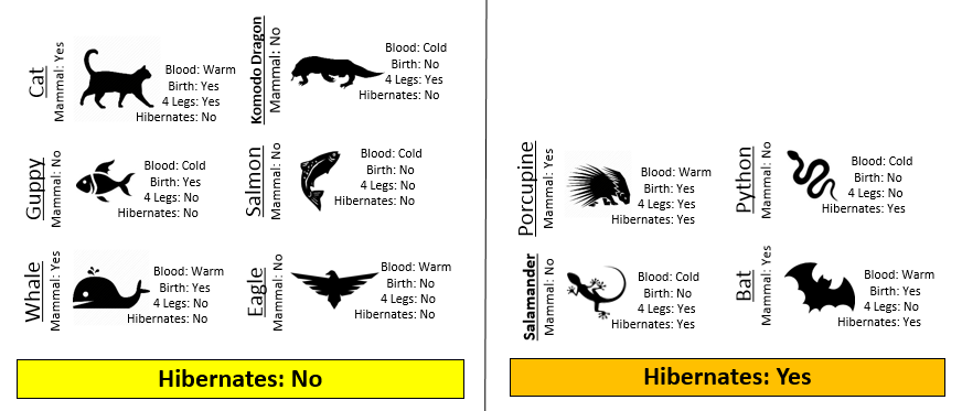Divide animal into two groups – Blooded = Warm and Blooded = Cold.
Step 2	Divide each respective group into – blooded = Warm and blooded = Cold.	Divide Blooded = Warm group into Gives Birth = Yes and Gives Birth = No.
Step 3	Divide Hibernates = No, Blooded = Warm into two additional groups, Gives Birth = Yes, and Gives Birth = No.

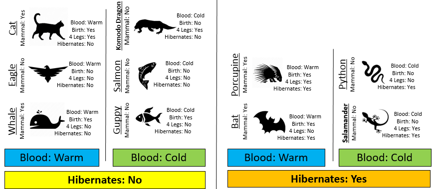
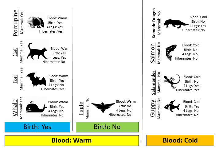
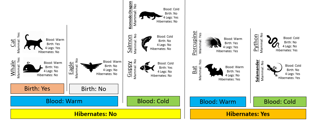
Comment: Rule #2 is a better rule as this rule is able to able to make valid predictions in less steps than Rule #1. Simplicity is a positive trait of a classification rule; however, a rule with optimal predictive ability is also important!

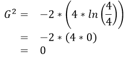
An algorithm will need to be able to identify which predictor variable is most advantages to use at any given step. The following quantity is used by R in the development of their classification trees.

where \(n_{i} = Number\ in\ node\ i\) and \(n_{i,\ k} = Number\ in\ node\ i\ that\ are\ of\ type\ j\).

Calculations for G:sup:`2` for each of the above rules

Iniital Value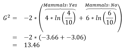

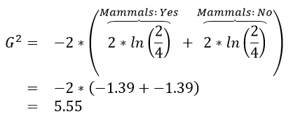
Rule #1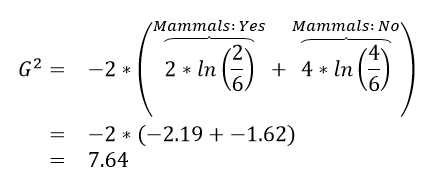

Rule #2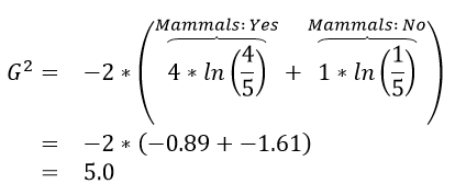

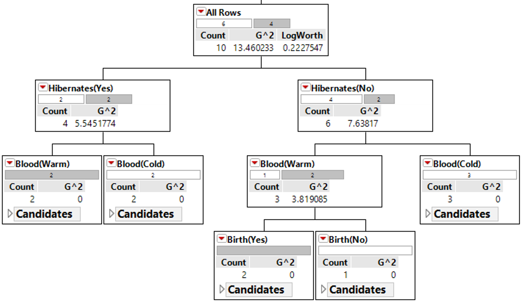
The initial or starting G² value is about 13.5. When using Rule #1, the combined G² value from the two nodes, i.e. Hibernates = Yes and Hibernates = No drops to (7.64 + 5.55) = 13.19. When using Rule #2, the combined G² value from Blood: Warm and Blood: Cold drops to (5.0 + 0.0) = 5.0. The drop in G² is considerable larger for Rule #2 – thus dividing the animal by Warm/Cold Blood is more advantageous.

Step	Rule #1	Rule #2
0	13.46	13.46
1	(7.64 + 5.55) = 13.19 2% drop	(5.0 + 0.0) = 5.0 63% drop
2	(3.81 + 0.0 + 0.0) = 3.81 72% drop	0.0+ 0.0) = 0.0 100% drop
3	(0.0+0.0+0.0+0.0) = 0.0 100% drop

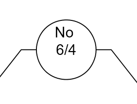
Classification rules are often arranged in a tree-type structure, hence the name Classification Tree.

	Appearance in JMP	Appearance in R via post() function
Step 0: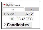
Step 1: Divide on Warm/Cold Blooded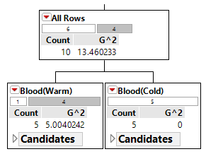
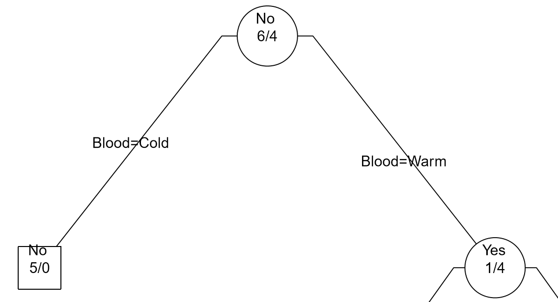Step 2: Divide Warm Blooded into Gives Birth Yes / No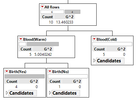

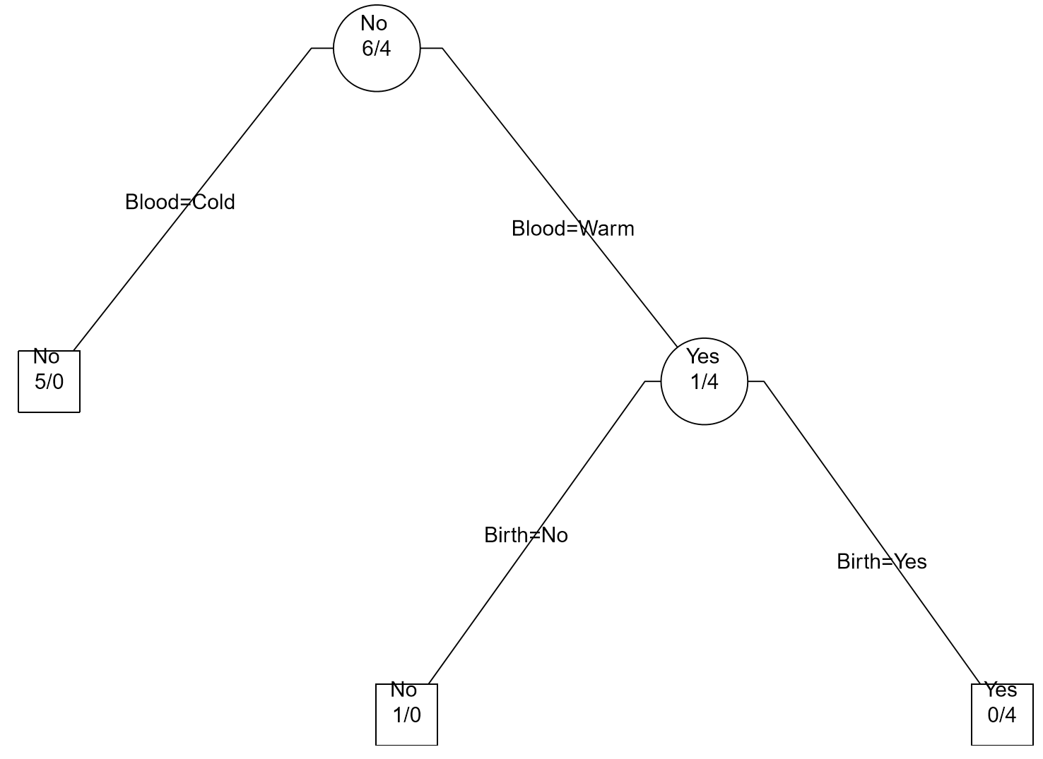As seen above, the Classification Tree for Rule #1 contains an additional layer that is not necessary.

Measuring Predictive Ability

Recall for Example 8.1, you were asked to construct a classification rule using the training dataset which included animals such as porcupine, salmon, bat, eagle, etc. After constructing your rule, a test dataset can be used to measure the overall quality of your predictions

• Training Dataset: Data used to build / construct a predictive model
• Test Dataset: Data used to measure the predictive ability of a model

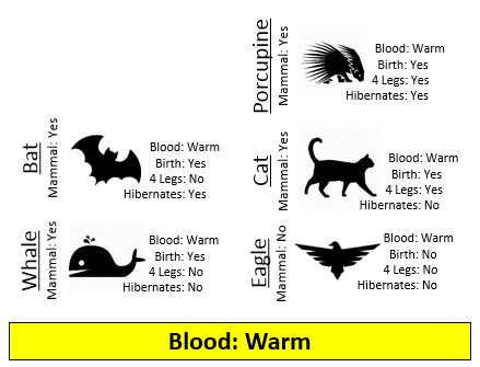
Consider the following animals that will be used as test cases to measure the quality of Rule #1 from Example 8.1.

Classification Rule #2	Using Rule #2 to make predictions

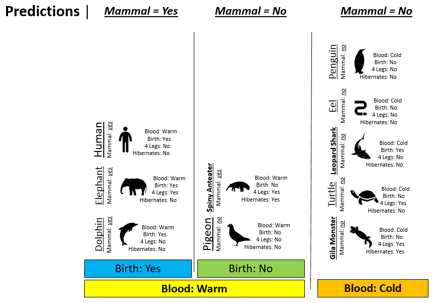Next, we must systematically check the validity of our predictions in each node. We can see that we have predicted the Spiny Anteater to be a Non-mammal when in fact it is a mammal.

There are a variety of measures that can be used to measure the quality of your prediction. One of the simplest measures is simply the misclassification rate. A misclassification matrix is commonly used to understand the nature of the misclassifications. The off-diagonal values in this matrix are cases that have been misclassified.

A misclassification rate can be computed. For Example 8.1, the misclassification rate for test dataset is 10%.

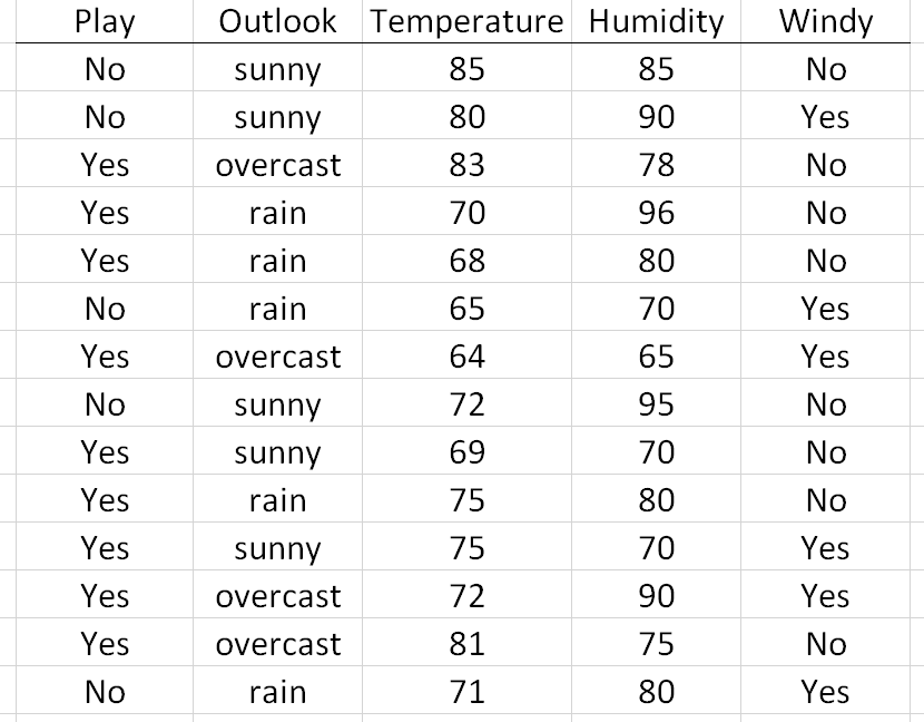
Example 8.2: Consider the following example where the goal is classify whether or not one should play golf on a given day. Response: Play Golf (Yes / No) Predictor variables: 1) Outlook (overcast, rain, sunny), 2) Temperature (OF), 3) Humidity (%), and 4) Windy (Yes, No).

Dealing with numerical predictors

The methodology for developing classification rules when using numerical predictors is similar to binary predictors. For numerical predictors, the algorithm will attempt to find an optimal cut-point that best separates the response variable. In a classification tree, all rules/decisions are binary (i.e. one either move to the left or right down the tree); thus, only a single cut-point is needed.

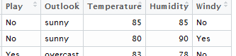
Suppose the classification rule is considering using Humidity to separate Play = Yes from Play = No.

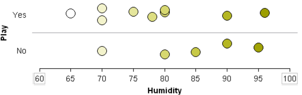
One can see that various cut-points will not be very useful in trying to separate Play = Yes from Play = No. Thus, humidity is likely not to appear early in the development of a classification tree.

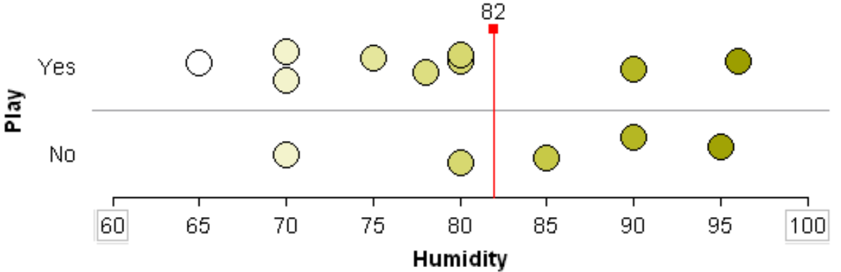
Will 82 work as a cut-point? No…

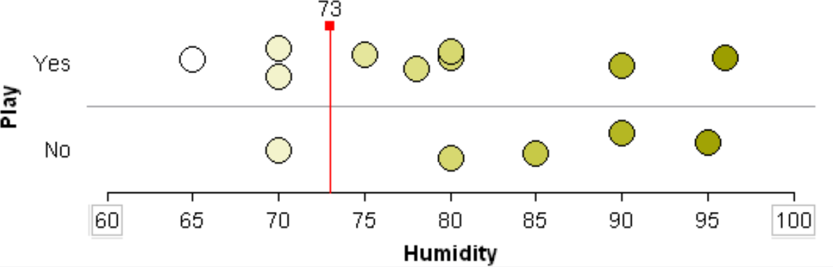
Will 73 work as a cut-point? No…

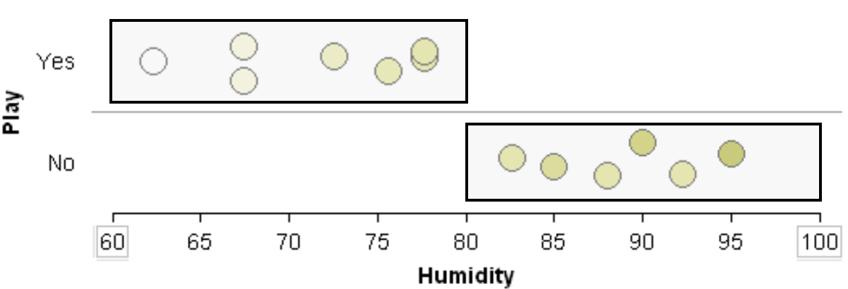
A situation in which Humidity would be a powerful predictor in separating Play = Yes from Play = No.

Dealing with categorical predictors that are not binary

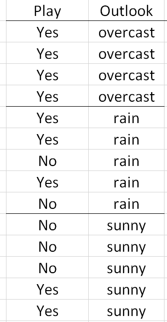
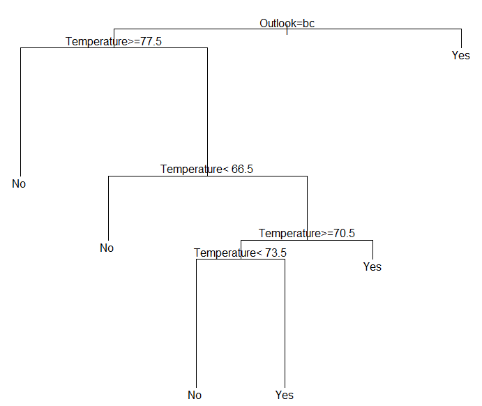
Consider again previous example that involved building a classification rule for playing golf. The Outlook predictor variable has three levels: overcast, rain, and sunny. As stated above, all rules/decisions are binary in a classification tree. Therefore, categorical predictors with multiple levels must be combined in a way to form binary sets that are disjoint.

Decisions rules must be binary; thus, the following is not allowed

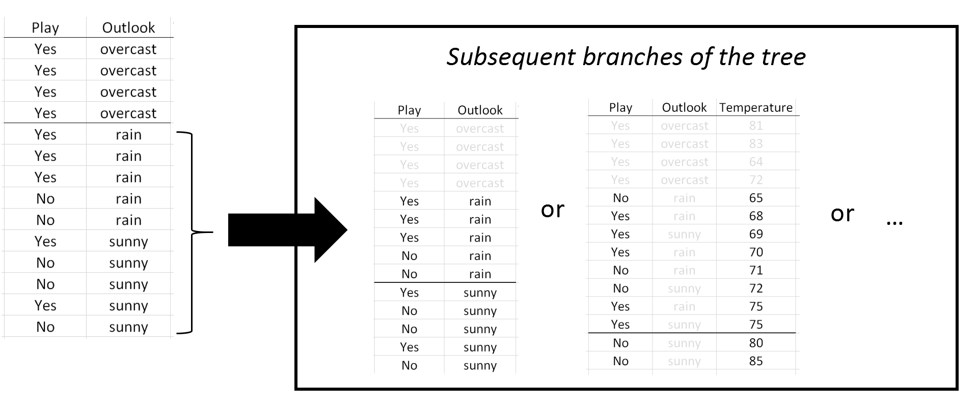
Here, the classification rule divided Outlook into two sets {overcast} and {rain, sunny}. In subsequent branches of the tree, Outlook could be used again to separate Play = Yes from Play = No or rules using other predictor variables, e.g. Temperature, may be more optimal.

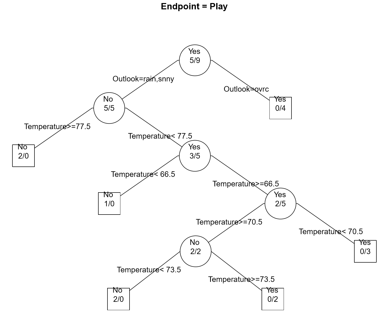
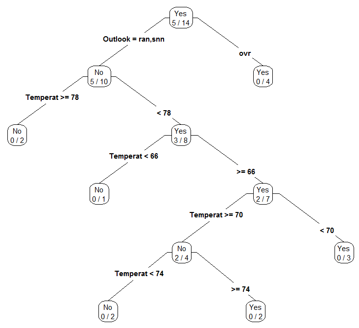
The complete classification tree fit using rpart() and post() function in R.

The Concept of Overfitting

Overfitting is a concept that naïve data scientists often overlook or are simple unaware of. Overfitting happens when a machine learning algorithm relies too much on the data being used to construct the predictive model. The most common way of identifying overfitting is a predictive model with good predictive ability for the data used to construct the predictive model, but a substantial decrease in predictive ability for new cases, i.e. cases in a test or holdout dataset.

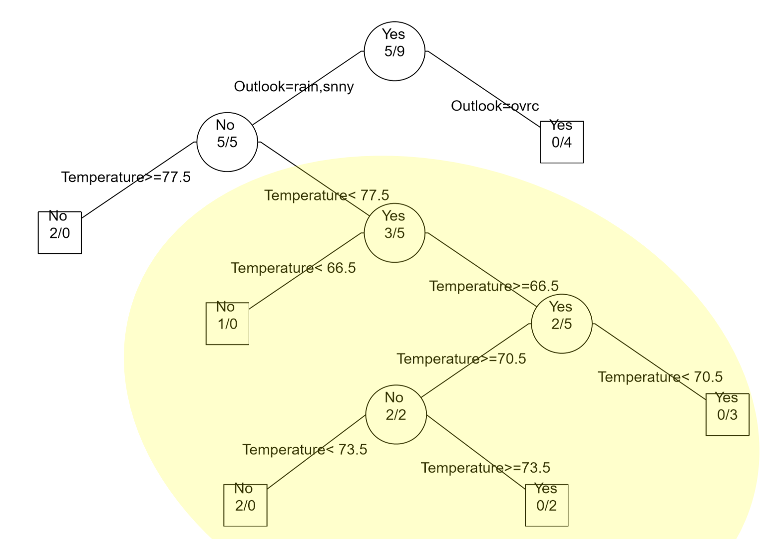
In the golf example (see Example 8.2) all available data was used to build the classification tree; thus, no data has been left out to test or verify the predictive ability of the model. However, other signals exist that overfitting may be taking place. For example, consider the lower branches of the classification tree provided for the golf data. Notice that very few observations are being selected for each branch – which may be a warning sign of overfitting. Finally, the golf example only had 14 observations; thus, overfitting is very likely to have occurred.

Another common problem in using trees is the over reliance on certain predictors. This appears to be the case for the golf example as Temperature is used repeated in this tree. To alleviate this problem, more complex algorithms, e.g. random forests, randomly select a set of predictors for consideration when building the predictive model.

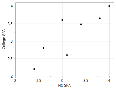
Overfitting may occur in any type of predictive model – not just classification trees. For example, suppose one wants to build a predictive model for College GPA using a person’s High School GPA. A predictive model that simply connects the dots would rely too much on the data being used to build the model.

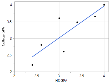
Relationship between College GPA and HS GPA	One possible predictive model is the trend line through the middle of the data
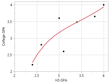
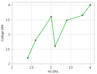
A second predictive model that is more flexible than the trend line provided above.	Connecting the dots would be considered overfitting as there is no residual error for this data and this model would have low predictive ability for a new prediction.

Classification Trees in R

We will begin with fitting the golf classification tree. The following code can be used to read in the golf.csv file.

#Reading in the golf data and viewwing

golf_df <- read.csv(file.choose(),header=T,stringsAsFactors = TRUE)

View(golf_df)

The classification tree will be constructing using the rpart() function that can be found in a package named rpart. The generic syntax for constructing a model has the following form.

Response ~ Predictor1 + Predictor2 + …

In the context of the golf example, the model would have the following form. The data should be passed into the rpart() function. The control option can be used to control the size of the tree – here a complete tree is being constructed for demonstration purposes.

Play ~ Outlook + Temperature + Humidity + Windy

#Using the rpart() function to fit the classification tree

library(rpart)

#Building the classification tree, using control option to build a complete tree

golf_tree <- rpart(Play ~ Outlook+Temperature+Humidity+Windy, data=golf_df, control = rpart.control(minsplit=1))

To plot the actual tree, two options are available 1) standard plotting, and 2) plotting via prp() function

#Plotting the tree plot(golf_tree) #Printing the text for the tree text(golf_tree) * Note*: Use levels(golf_df$Outlook) to identify labels.

# Using the rpart.plot package and the prp() plotting function library(rpart.plot) prp(golf_tree,type=4,extra=3)

The summary() function can be used to view details of the classification tree.

> summary(golf_tree)

Call:

rpart(formula = Play ~ Outlook + Temperature + Humidity + Windy,

data = golf_df, control = rpart.control(minsplit = 1))

n= 14

CP nsplit rel error xerror xstd

1 0.20 0 1 1.0 0.3585686

2 0.01 5 0 1.6 0.3703280

Variable importance

Temperature Outlook Windy

76 20 4

Node number 1: 14 observations, complexity param=0.2

predicted class=Yes expected loss=0.3571429 P(node) =1

class counts: 5 9

probabilities: 0.357 0.643

left son=2 (10 obs) right son=3 (4 obs)

Primary splits:

Outlook splits as RLL, improve=1.4285710, (0 missing)

Humidity < 82.5 to the right, improve=0.9174603, (0 missing)

Temperature < 84 to the right, improve=0.8901099, (0 missing)

Windy splits as RL, improve=0.4285714, (0 missing)

:

etc…

Next, consider the construction of a classification tree for the mammals dataset. The first step is to read in the mammals data.

#Reading in the mammals data and viewing the data

mammals_df <- read.csv(file.choose(),header=T,stringsAsFactors = TRUE)

View(mammals_df)

Recall, this dataset is divided into two parts 1) training datasets and 2) test dataset. The predictive model should be built using only the training cases.

#Fitting the classification tree to the training data, filter() from dplyr package is being used to fit only the Training dataset

library(dplyr)

#Fitting a complete tree for the training data

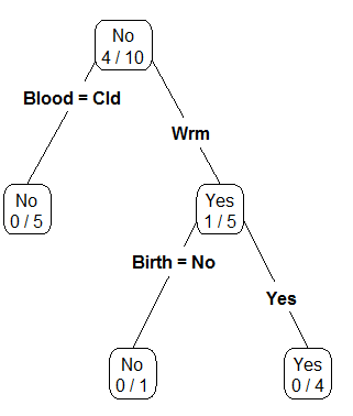
mammals_tree <- rpart(Mammal~Blood+Birth+X4Legs+Hibernates, data=filter(mammals_df,Designation == “TrainingData”), control=rpart.control(minsplit = 1))

#Plotting the classification tree

prp(mammals_tree,type=4,extra=3)

This data contains test cases; thus, predictions can be made using the classification tree to evaluate the predictive ability of this model.

#Gettting the Test Dataset via filter()

> filter(mammals_df,Designation==”TestData”)

Name Mammal Blood Birth X4Legs Hibernates Designation

1 Human Yes Warm Yes No No TestData

2 Pigeon No Warm No No No TestData

3 Elephant Yes Warm Yes Yes No TestData

4 Leopard Shark No Cold Yes No No TestData

5 Turtle No Cold No Yes No TestData

6 Penguin No Cold No No No TestData

7 Eel No Cold No No No TestData

8 Dolphin Yes Warm Yes No No TestData

9 Spiny Anteater Yes Warm No Yes Yes TestData

10 Gila Monster No Cold No Yes Yes TestData

The generic predict() function in R can be used to make predictions. The test dataset will be passed into the predict() function. It should be noted that the structure of the test data.frame should be the same as the training data.frame. The use of filter() ensure that this will be the case. The type=”class” should be specified in the predict() function to ensure proper labeling of the output.

> mammal_predict <- predict(mammals_tree,newdata=filter(mammals_df,Designation==”TestData”),type=”class”)

The predicted outcomes for these 10 animals are shown here.

> mammal_predict

1 2 3 4 5 6 7 8 9 10

Yes No Yes No No No No Yes No No

Levels: No Yes

The predicted outcomes should be compared against the actual outcomes. We can see that case #9, i.e. the Spiny Anteater, has been misclassified. This is the only animal to be misclassified in the test dataset.

> filter(mammals_df,Designation==”TestData”)$Mammal

[1] Yes No Yes No No No No Yes Yes No

Levels: No Yes

A custom function, named Misclassify(), is created to automatically print the misclassification matrix and to compute the misclassification rate for the predictions in the test / holdout dataset.

Misclassify = function(Predicted,Actual) {

temp <- table(Predicted,Actual)

cat(“\n”)

cat(“Table of Misclassification\n”)

cat(“(rows: predicted, columns: actual)\n”)

print(temp)

cat(“\n”)

numcorrect <- sum(diag(temp))

numincorrect <- length(Actual) - numcorrect

mcrate <- numincorrect/length(Actual)

cat(paste(“Misclassification Rate = ”,100*round(mcrate,3),”%”))

cat(“\n”)

}

Using the Misclassify() function to evaluate the quality of the prediction for the mammals test dataset.

#Using the misclass() function to obtain the

> Misclassify(mammal_predict,filter(mammals_df,Designation==”TestData”)$Mammal)

Table of Misclassification

(rows: predicted, columns: actual)

Actual

Predicted No Yes

No 6 1

Yes 0 3

Misclassification Rate = 10 %

Example 8.3

Consider the following example in which mushrooms are to be classified into two categories – edible and poisonous. For this example, there are about 20 predictor variables available for use. These predictor variables happen to be all categorical in nature. Variable/feature descriptions are provided in the following table.

Edible

Poisonous

Variable / Feature	Description
Y:Poisonous	edible=e,poisonous=p
X1:CapShape	bell=b,conical=c,convex=x,flat=f,knobbed=k,sunken=s
X2:CapSurface	fibrous=f,grooves=g,scaly=y,smooth=s
X3:CapColor	brown=n,buff=b,cinnamon=c,gray=g,green=r,pink=p,purple=u, red=e,white=w,yellow=y
X4:HasBruises	yes=y, no=n
X5:Odor	almond=a,anise=l,creosote=c,fishy=y,foul=f,musty=m,none=n,pungent=p, spicy=s
X6:GillAttachment	attached=a,descending=d,free=f,notched=n
X7:GillSpacing	close=c,crowded=w,distant=d
X8:GillSize	broad=b,narrow=n
X9:GillColor	lack=k,brown=n,buff=b,chocolate=h,gray=g,green=r,orange=o,pink=p,purple=u,red=e, white=w,yellow=y
X10:StalkShape	enlarging=e,tapering=t
X11:StalkSurfaceAboveRing	ibrous=f,scaly=y,silky=k,smooth=s
X12:StalkSurfaceBelowRing	ibrous=f,scaly=y,silky=k,smooth=s
X13:StalkColorAboveRing	brown=n,buff=b,cinnamon=c,gray=g,orange=o,pink=p,red=e,white=w,yellow=y
X14:StalkColorBelowRing	brown=n,buff=b,cinnamon=c,gray=g,orange=o,pink=p,red=e,white=w,yellow=y
X15:VeilType	partial=p,universal=u
X16:VeilColor	brown=n,orange=o,white=w,yellow=y
X17:RingNumber	none=n,one=o,two=t
X18:RingType	cobwebby=c,evanescent=e,flaring=f,large=l,none=n,pendant=p,sheathing=s,zone=z
X19:SporePrintColor	black=k,brown=n,buff=b,chocolate=h,green=r,orange=o,purple=u,white=w,yellow=y
X20:Population	abundant=a,clustered=c,numerous=n,scattered=s,several=v,solitary=y
X21:Habitat	grasses=g,leaves=l,meadows=m,paths=p,urban=u,waste=w,woods=d

*Getting this data into R using the read.csv() function. This data has 8124 cases and 22 variables (1 response variable and 21 predictor variables).

mushrooms_df <- read.csv(file.choose(),header=T, stringsAsFactors = TRUE)

View(mushrooms_df)

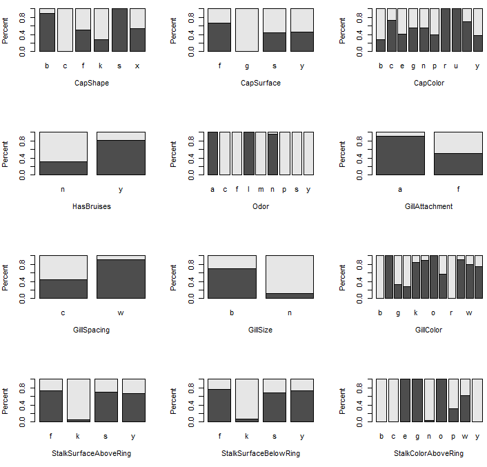
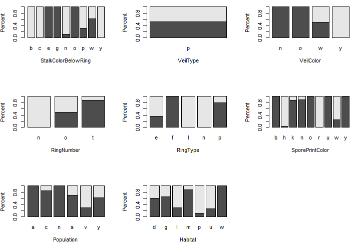
Some preliminary plots…

par(mfrow=c(4,3))

barplot(prop.table(table(mushrooms_df$Poisonous,mushrooms_df$CapShape),2),ylab=”Percent”,xlab=”CapShape”)

To begin, let us first consider the relationship between Poisonous and each of the predictor variables. The following mosaic plots will help determine which predictor variables will be useful in separating the edible from poisonous mushrooms.

Legend: Dark gray = edible, light gray is poisonous.

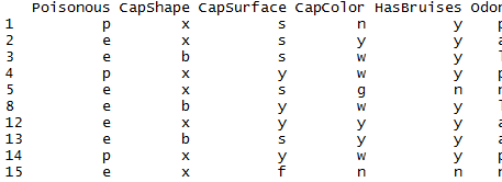
This dataset contains several thousand observations. Therefore, this data will be divided into a Training dataset and a test / holdout dataset. Random division of the observations is done here to reduce the potential for bias.

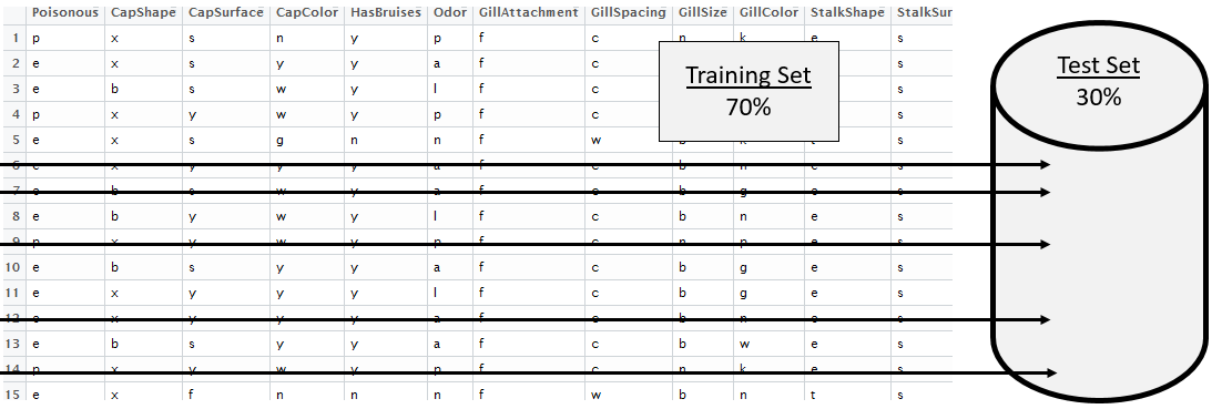
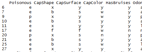
In R, getting a random selection of 30% of the 8124 cases which will be used as the test cases.

> test_rows <- sample(1:8124,0.30*8124,replace=F)

> head(sort(test_rows),20)

[1] 6 7 9 10 11 17 20 21 25 27 29 39 43 50 53 58 62 64 65 67

Syntax for referencing training dataset mushrooms_df[-test_rows,]	Training Dataset
Syntax for referencing test dataset mushrooms_df[test_rows,]	Test Cases

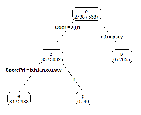
Fitting a classification tree for the mushroom data using only the training rows from the data.frame.

#Fitting a classification tree

> mushrooms_tree <- rpart(Poisonous ~ ., data=mushrooms_df[-test_rows,])

#Plotting the tree, using prp() function which is part of rpart.plot package

> library(rpart.plot)

> prp(mushroom_tree, type=4, extra=3)

Note: The names() function can be used to help identify shortened names. The levels() command might also be necessary to identify the levels for a particular variable, e.g. binary outcomes Yes / No, maybe labeled as a/b or as y/n.

> names(mushrooms_df)

[1] “Poisonous” “CapShape” “CapSurface” “CapColor”

[5] “HasBruises” “Odor” “GillAttachment” “GillSpacing”

[9] “GillSize” “GillColor” “StalkShape” “StalkSurfaceAboveRing”

[13] “StalkSurfaceBelowRing” “StalkColorAboveRing” “StalkColorBelowRing” “VeilType”

[17] “VeilColor” “RingNumber” “RingType” “SporePrintColor”

[21] “Population” “Habitat”

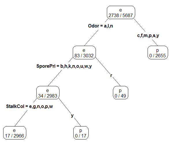
*Fitting a slightly larger tree – this is done by reducing the cp value and/or the minsplit value which are passed into the rpart() function through the control parameter.

mushroom_tree2 <- rpart(Poisonous ~ ., data=mushrooms_df[-test_rows,], control=rpart.control(cp=0.005,minsplit = 3))

prp(mushroom_tree2,type=4,extra=3)

Finally, the misclassification rate for each rule is computed using the previously used Misclassify() function.

#Misclassification Rate for first tree

Table of Misclassification

(rows: predicted, columns: actual)

Actual

Predicted e p

e 1259 14

p 0 1164

Misclassification Rate = 0.6 %

#Getting the misclassification rate for second tree – the more complex tree

Table of Misclassification

(rows: predicted, columns: actual)

Actual

Predicted e p

e 1259 7

p 0 1171

Misclassification Rate = 0.3 %

Tasks

1. Suppose you work for small upstart company who is considering extending credit to customers through a store credit card, e.g. Kohls Card, Scheels Card, etc. You have been asked to investigation whether or not one can reliably predict the credit risk of a customer given a set of predictor variables about this customer.

   Download the GermanCreditRisk data from the course website. The response variable of interest here is Credit Risk (Good / Bad). The predictor variables are: CreditHistory, CheckingAccount - level of money in checking account, SavingsAccount – level of money in savings account, Age of customer, Housing, Employment, JobSkill, OtherCreditFromUs – does customer have existing credit account with us, TotNumberCreditAccounts – total number of credit accounts, OtherDebtors, Purpose, CreditAmount – amount of credit to be extended, RepaymentPercent – monthly payment as a percentage of monthly disposable income.

   1. After reading in the data, create mosaic plots for each of the predictor variables that are categorical in nature, i.e. CreditHistory, CheckingAccount, etc. Code has been provided for plotting CreditRisk vs. CreditHistory, this code can be edited for the other categorical predictor variables.

   #Reading in the dataset

   CreditRisk_df <- read.csv(file.choose(), header=T, stringsAsFactors = TRUE)

   #View of data.frame

   View(CreditRisk_df)

   #Creating a barplot for CreditHistory

   barplot(prop.table(table(CreditRisk_df$CreditRisk,CreditRisk_df$CreditHistory),2))

1. Next, create plots to investigate the relationship between CreditRisk and the numeric variables – Age and CreditAmount. Again, code has been provided for Age and can be edited to plot relationship for CreditAmount.

   #Loading the lattic() package

   library(lattice)

   #Using a densityplot to see if there is a shift in Age between CreditRisk

   densityplot(~Age, data=CreditRisk_df, groups=CreditRisk, plot.points=FALSE, auto.key=TRUE)

1. Why type of plot, barplot() or densityplot(), should be used to understand the relationship between CreditRisk and TotNumberCreditAccounts and CreditRisk and RepaymentPercent? Try both a barplot() and densityplot(). Which plot is better? Discuss.

2. Consider the plots made in part a., part b, and part c. Which predictor variables appear to best separate CreditRisk = Good from CreditRisk = Bad? Discuss.

3. Next, use the rpart() function in R to build a classification tree for predicting CreditRisk. Plot your classification tree.

4. Which predictor variable does your classification tree use early one? Which predictor variables are used later in building the tree? What does it mean, in a practical sense, when a variable is used early in the classification rule (vs. later in a classification tree)? Discuss.

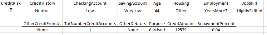
5. Suppose a new customer is seeking credit with the following profile. Use your classification tree to make a CreditRisk prediction for this customer. Should we extend credit to this customer? Discuss.

   

1. For the second task, build a classification rule to determine whether or not a women’s a breast biopsy is cancerous (malignant, denoted M in dataset) or not (benign, denoted B in dataset). There are 10 predictor variables / features that are measurements regarding various characteristics of the cells examined. These features include: Radius, Texture, Perimeter, Area, Smoothness, Compactness, Concavity, ConcavePts, Symmetry, and FracDim.
   1. Divide this dataset into a training set (70%) and test set (30%).
   2. Build two different classification trees – a simple tree and a second more complex tree.
   3. Make predictions for the test set using each rule. What is the misclassification rate for each rule?
   4. Which predictor variables are most important in your classification tree? Discuss.
   5. Provide a description (for a doctor) that would describe how to make a prediction using your classification tree?