6.7. Writing Custom Functions
Before we discussing writing new functions in R, let’s examine an existing function more closely. For more insight into the coding behind the median() function, consider the following R commands and output.
> median
function (x, na.rm = FALSE)
UseMethod(“median”)
<bytecode: 0x000000000b265d20>
<environment: namespace:stats>
> methods(median)
[1] median.default
> median.default
function (x, na.rm = FALSE)
{
if (is.factor(x) || is.data.frame(x))
stop(“need numeric data”)
if (length(names(x)))
names(x) <- NULL
if (na.rm)
x <- x[!is.na(x)]
else if (any(is.na(x)))
return(x[FALSE][NA])
n <- length(x)
if (n == 0L)
return(x[FALSE][NA])
half <- (n + 1L)%/%2L
if (n%%2L == 1L)
sort(x, partial = half)[half]
else mean(sort(x, partial = half + 0L:1L)[half + 0L:1L])
}
When determining how to use this function, note that this function contains two arguments: x and na.rm. For more information on these arguments, you should review the help documentation for median.
> help(“median”)
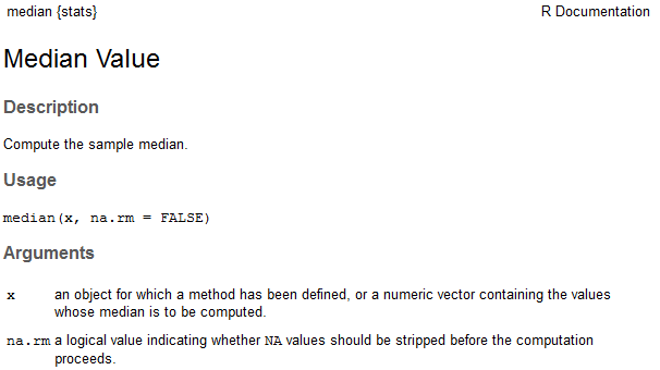
Notice that by default, the na.rm argument is set to FALSE. This means that the following arguments both return the same result:
> #Creating a vector of ages that represents typical ages for working adults
> ages <- seq(18,65)
>
> #Taking a (random) sample of 10 ages – with replacement
> mydata <- sample(ages,size=10,replace=TRUE)
> mydata
[1] 47 42 54 46 49 21 32 56 21 26
>
> #Setting a seed to ensure we get the same random sample
> set.seed(987654321)
>
> mydata <- sample(ages,size=10,replace=TRUE)
> mydata
[1] 35 56 44 26 49 24 43 34 51 53
>
> #Compute median of x
> median(mydata)
[1] 43.5
>
> #Creating some missingness, replace the 5th number with NA
> mydata[5] <- NA
> mydata
[1] 35 56 44 26 NA 24 43 34 51 53
> median(mydata)
[1] NA
> median(mydata,na.rm=TRUE)
[1] 43
The previous example gives us some insight into how functions are written with arguments that are called within R. You can learn a lot about R programming by examining the code behind functions that were written by others. The remainder of this handout provides an introduction to the basics of writing your own functions in R.
6.7.1. ***
*WRITING NEW FUNCTIONS IN R*
One of the advantages of using a scripting language like R is the ability to write your own functions (or to modify existing functions). An R programmer can define their own functions using the function() and return() functions.
Example 1: Creating a simple function
Note that the sum() function already exists in R and can be used to add two numbers; for illustrative purposes, however, we will write our own simple function to do this. The parameters (or values) being used by this function have been generically named param1 and param2.
> #Add two function
> Addtwo <- function(param1,param2){
- param1 + param2
- }
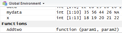
This new function will be listed in your Global Environment under Functions.
To call the function, enter the following at the prompt.
> Addtwo(param1=3,param2=9)
[1] 12
You can shortcut the function call as follows (dropping the parameter names).
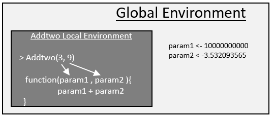
> Addtwo(3,9)
[1] 12
* *R uses a local environment for function parameters. For example, if param1 exists in the global environment and also in the local environment, R will use the value in the local function environment.
> param1 <- 10
> Addtwo(param1=3,param2=9)
[1] 12
Suppose a parameter does not exist in the local function environment, then R will search and use this parameter if it exists in the global environment.
> #Add three function
> Addthree <- function(param1,param2){
- param1 + param2 + param3
- }
> #Using the Addthree function
> param3 <- 100
> Addthree(param1=3,param2=9)
[1] 112
Example 2: Creating a simple function – with default values
Default vales can be specified for a function. Parameter specification is done when specifying arguments for the function.
> #Add two function with default value for param2
> Addtwo <- function(param1,param2=100){
- param1 + param2
- }
> #Usage of this version, only param1 being specified in function call
> Addtwo(param1=10)
[1] 110
Specify a default value for the first parameter.
> #Add two function with default value for param1
> Addtwo <- function(param1=-500,param2){
- param1 + param2
- }
> #Usage of this version
> Addtwo(,param2=5)
[1] -495
> Addtwo(,5)
[1] -495
The following will not work, as this is setting param1 = 5, and no value has been specified for param2.
> Addtwo(5)
Error in Addtwo(5) : argument “param2” is missing, with no default
*Example 3: Creating a function to compute multiple quantities*
Next, suppose you want to write a function in R to both find the difference between two values and the ratio of those two values. You may start with the following.
> Myfunction <- function(a,b){
- a-b
- a/b
- }
> #Using this function
> MyFunction(4,2)
[1] 2
Note that the function returns the result of only the last of the computations. To report all of the results, you can use the return statement as shown below.
> MyFunction <- function(a,b){
- return(c(a-b, a/b ))
- }
> MyFunction(4,2)
[1] 2 2
Finally, note that it may be more useful to assign names to the values calculated and to return a more flexible data type (such as a list object) to provide more information about the calculations that have been performed. The following programming statements return the results in a list.
> MyFunction <- function(a,b){
- Result1 = a-b
- Result2 = a/b
- return(list(Difference=Result1,Ratio=Result2))
- }
> MyFunction(4,2)
$Difference
[1] 2
$Ratio
[1] 2
6.7.2. ***
> ?average
No documentation for ‘average’ in specified packages and libraries:
you could try ‘??average’
- s = sum(x)
- avg = s/length(x)
- return (avg)
- }
Note that this function can now be applied to calculate the average of any vector in R.
> average(x)
[1] 0.4783486
* Example 5: Dealing with missing values*
Missing values should be considered when writing custom functions. For example, the average() function written above will not work with missingness present.
> x[2]<-NA
> x
[1] 0.36888095 NA 0.54802340 0.17993140 0.65435477 0.12500433 0.52510142 0.35084670 0.70311331
[10] 0.73129676 0.61784387 0.52065692 0.75065050 0.58954068 0.65485598 0.07954121 0.30900394 0.79808945
[19] 0.07708921 0.17460408
> average(x)
[1] NA
Missing values can be dealt with easily in this simple case by adding na.rm=TRUE to the sum() function. In addition, na.omit() will be used to omit any missing values when computing the length of the vector.
> average <- function(x){
- s = sum(x, na.rm=TRUE)
- avg = s/length(na.omit(x))
- return (avg)
- }
> average(x)
[1] 0.4609699
A check to make sure NA is being properly ignored. The x[-2] syntax simply removes the second element to x.
> average(x[-2])
[1] 0.4609699
* Example 6: Modifying the summary() function*
R allow us to expand upon existing functions. Consider the following in which the summary() function is being applied to a data.frame.
> set.seed(987654321)
> x<-runif(20,0,1)
> summary(x)
Min. 1st Qu. Median Mean 3rd Qu. Max.
0.07709 0.27670 0.53660 0.47830 0.66690 0.80850
We will now add to the standard list of summaries the standard deviation, mean absolute deviation, and the count. The following code will add these summaries to standard output provided by the summary() function.
> num.summary <- function(x){
- original = summary(x)
- stdev = sd(x,na.rm=TRUE)
- mean.abs.dev = mean(abs(na.omit(x)-mean(na.omit(x))))
- n=length(na.omit(x))
- list(c(original,”Std Dev” = stdev, “MAD” = mean.abs.dev,”Count”=n))
- }
The modified summary function includes the additional summaries.
> num.summary(x)
[[1]]
Min. 1st Qu. Median Mean 3rd Qu. Max. Std Dev MAD Count
0.0770900 0.2767000 0.5366000 0.4783000 0.6669000 0.8085000 0.2498250 0.2161887 20.0000000
Finally, note that you could change the layout of the output. The paste() and round() functions are used here for writing to the screen and for rounding output.
> num.summary <- function(x){
- Min = summary(x)[1]
- Q1 = summary(x)[2]
- Q2 = summary(x)[3]
- Q3 = summary(x)[5]
- Max = summary(x)[6]
- Mean = summary(x)[4]
- s = sd(x,na.rm=TRUE)
- mean.abs.dev = mean(abs(na.omit(x)-mean(na.omit(x))))
- n=length(na.omit(x))
- cat(paste(“Min: ”, Min))
- cat(“\n”)
- cat(paste(“Q1: ”, Q1))
- cat(“\n”)
- cat(paste(“Median: ”, Q2))
- cat(“\n”)
- cat(paste(“Q3: ”, Q3))
- cat(“\n”)
- cat(paste(“Max: ”, Max))
- cat(“\n”)
- cat(paste(“Mean: ”, Mean))
- cat(“\n”)
- cat(paste(“Standard Deviation: ”, round(s,4)))
- cat(“\n”)
- cat(paste(“Mean Absolute Deviation: ”, round(mean.abs.dev,4)))
- cat(“\n”)
- cat(paste(“Sample Size: ”, round(n,0)))
- }
The output with custom printing.
> num.summary(x)
Min: 0.07709
Q1: 0.2767
Median: 0.5366
Q3: 0.6669
Max: 0.8085
Mean: 0.4783
Standard Deviation: 0.2498
Mean Absolute Deviation: 0.2162
Sample Size: 20
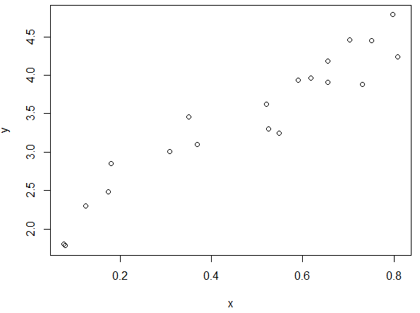
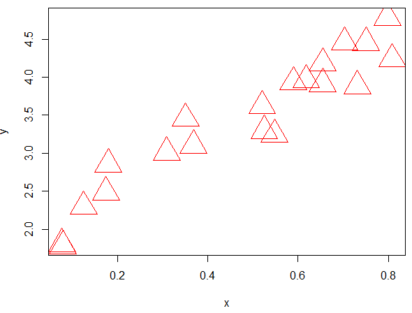
*Example 7: Modifying the plot() function*
Consider the following data and its associated plot.
> #Getting a vector of random data
> set.seed(987654321)
> x<-runif(20,0,1)
> y<-2 + 3*x + runif(20,-0.5,0.5)
Suppose you want the plot() function to use a very large triangle plotting character that is red. The plot() function can be modified as follows. R allows you to pass an unspecified number of parameters to a function using the … notation. Note: One should carefully consider the order of the arguments in the list when using the … notation.
> myplot <- function(..., pch.new=2, col.new=”red”, cex.new=4.0 ) {
- plot(..., pch=pch.new, col=col.new, cex=cex.new )
- }
>
> #USing the new plottign function
> myplot(x,y)
Tasks:
- Recall that the formula for a sphere is 4⁄3πr3. Write a function named sphere.volume that returns the volume of a sphere when given the radius r as a parameter. Then, call the function to return the volume of a sphere with a radius of 5. Call the function again to return the volume of a sphere with a radius of 10.
- Write a function named myplot which calls the plot() function but uses a blue open circles as the default plotting symbol. Create a plot using your new myplot() function.